 |
About AMP Lab Projects Downloads Publications People Links
Project - The Self-Reconfigurable Camera Array
| Motivation and Goal |
Image-based rendering (IBR) has attracted much research interest recently. By capturing many images of a scene, IBR is capable of rendering realistic 3D scenes without much scene geometry information. One difficulty in IBR is the huge amount of data to store or transmit, which makes it extremely difficult to capture and render scenes that have dynamic content in real-time.
In this project, we want to build a camera array for capturing and rendering dynamic scenes. The system is built upon the following goals: First, we need tens of cameras in the array. Dense cameras allow us to perform rendering at a reasonably good quality without prior knowledge of scene geometry. It also provides a larger viewing space for the user to navigate. Second, we want to perform capturing and rendering all in a real-time. This is a very challenging goal considering so many cameras are to be handled at the same time. Third, we want to make the camera array self-reconfigurable. Reconfiguration of the cameras' position and direction is important because we can use fewer cameras while maximizing the output rendering quality. Mobile cameras can move around in order to best perform the task, for instance, to render better quality images for IBR. Finally, the system need to be low-cost for obvious reasons. The overall cost of our system is around $22,000 U.S. dollars.
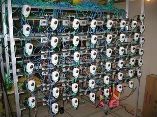
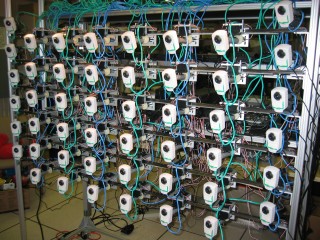
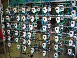
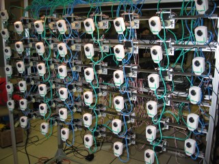
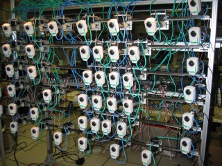
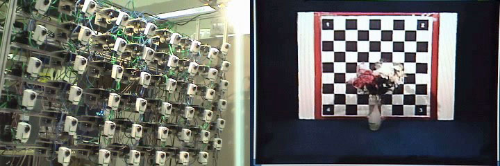
Our system is composed of inexpensive off-the-shelf components. There are 48 Axis 205 network cameras mounted on 6 linear guides. Each camera can capture up to 640x480 pixel2 images at rates of up to 30 fps. The cameras have built-in HTTP servers, which respond to HTTP requests and can stream motion JPEG sequences. The JPEG image quality is controllable. The cameras are connected to the computer through 1Gbps Ethernet cables.
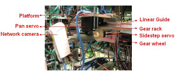
A close view of a camera unit is shown above. The camera is attached to a pan servo, which is a standard servo capable of panning through a 90 degree range. They are mounted on a platform, which is equipped with another sidestep servo. The sidestep servo has been modified so that it can rotate continuously. A gear wheel is attached to the sidestep servo, which allows the platform to move horizontally with respect to the linear guide. The gear rack is added to avoid slippery during the motion. Therefore, the cameras have two degrees of freedom, pan and sidestep. However, at the most left and right column of the camera array, the 12 cameras have fixed positions and can therefore only pan.
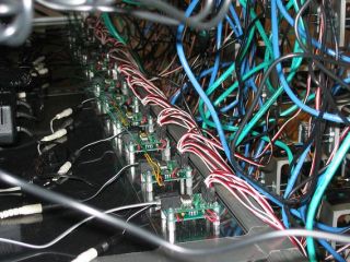
The servos are controlled by Scott Edwards Electronics Inc.'s popular Mini SSC II servo controller. Each controller manages no more than 8 servos (either standard or modified servos). A nice feature of the Mini SSC II controllers is that they can be chained to control up to 255 servos. All linked controllers can communicate with the computer through a single serial cable. In the current system, we use altogether 11 Mini SSC II controllers to control 84 servos (48 pan servos, 36 sidestep servos).
Unlike some large camera array systems available today (the
Stanford multi-camera array,
the MIT
distributed light field camera and
the CMU 3D
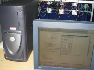
room), our whole system uses only one computer. The computer is an Intel
Xeon 2.4 GHz dual processor machine with 1GB of memory and a 32 MB NVIDIA
Quadro2 EX graphics card. This computer is responsible for grabbing images from
the camera array, performing JPEG image decoding, correcting camera lens distortions,
render novel views interactively, and control the motion of the cameras.
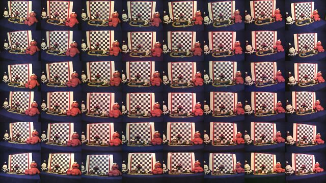
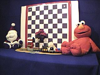
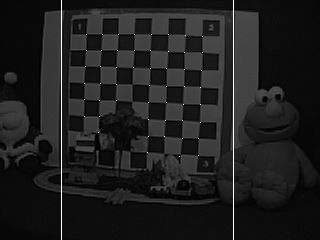
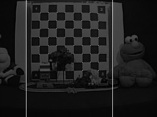
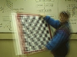
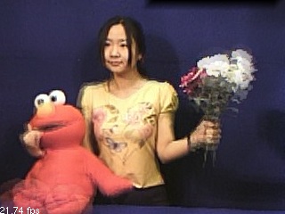
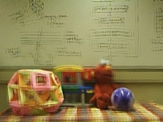
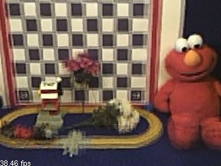
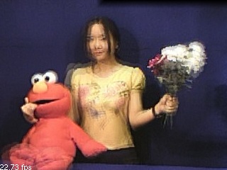
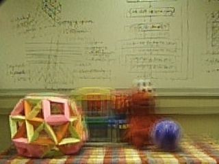
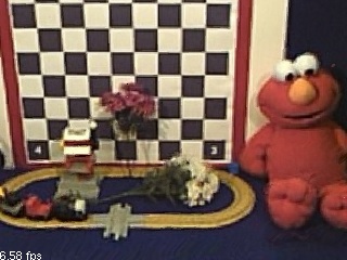
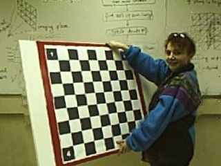
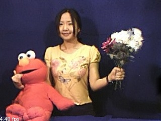
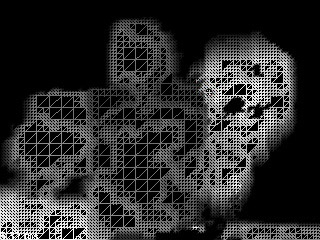
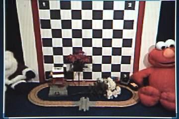
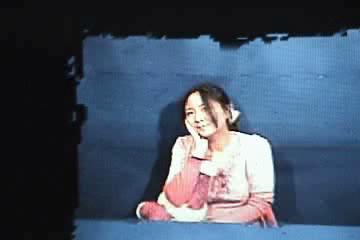
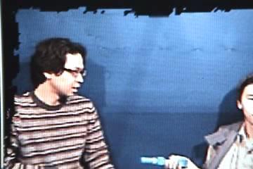
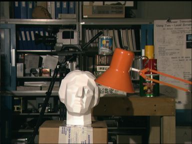
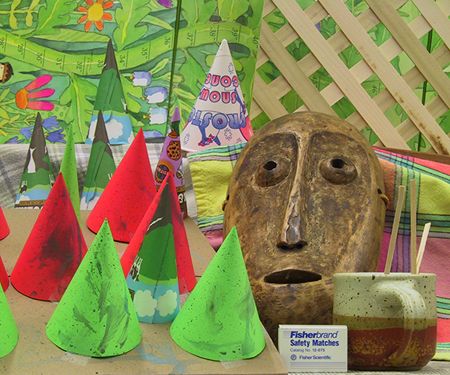
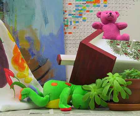
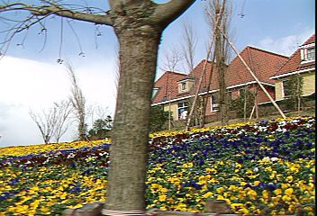
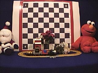
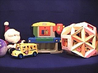
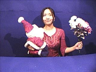
The above figures shows some of the images captured by our camera array at resolution 320x240. In these examples, the horizontal spacing between cameras is about 20 cm and the vertical spacing is about 15 cm. The disparity between images is fairly large. The images captured by the cameras are compressed with quality factor 30 (0 being the best, 100 being the worst) and transmitted to the computer. Each captured image occupies about 12-18 KBytes. In a 1 Gbps Ethernet connection, 48 cameras can send such JPEG image sequences to the computer simultaneously at 25-30 fps, which is satisfactory. In the latter examples, we operate the cameras at resolution 320x240 and 10 fps.
From the above images, one can see that the captured image set is very challenging due to the large color variations, lens distortion, JPEG compression artifacts, etc. Moreover, the Axis 205 cameras cannot be simultaneously triggered (although their clocks can be synchronized through an NTP server). We employ a triple buffering scheme which guarantees that the rendering process will always use the most recently arrived images at the computer for synthesis.
| Camera Calibration |
We use a large planar calibration pattern for the calibration of the cameras. The internal parameters of the cameras are calibrated separately using Bouguet's calibration toolbox. The external parameters of the cameras are calibrated on the fly. The checker board corners are extracted at a coarse level through two linear filters. Sub-pixel accuracy of the corners is then obtained iteratively by finding the saddle points. To obtain the 6 external parameters (3 for rotation, 3 for translation), we use the Levenberg-Marquardt method available in MinPack for nonlinear optimization.
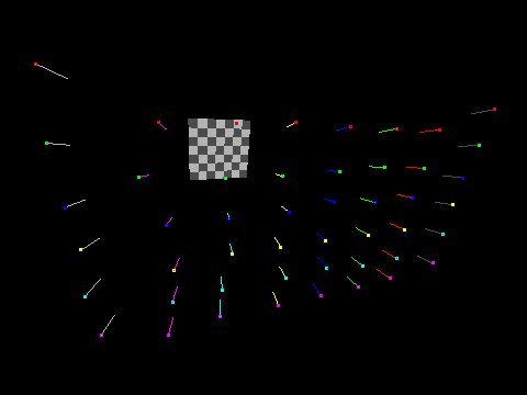
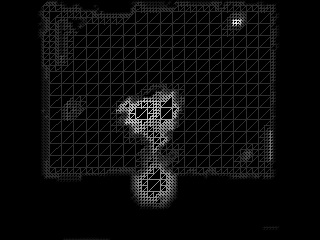
The above figure shows the results of our on-the-fly calibration algorithm. Each color dot represents the location of a camera, and its attached line segment represents the view direction of the camera. On our computer, this calibration process runs at about 150-200 fps with one processor. As long as the cameras are not all moving simultaneously, we can calibrate them in real-time.
| Real-Time Rendering |
We developed an algorithm for the rendering of dynamic scenes with our camera array in real-time. In short, we reconstruct the geometry of the scene as a multi-resolution 2D mesh with depths on its vertices. The 2D mesh is positioned on the imaging plane of the virtual view, thus the geometry is view-dependent. The depths of the vertices are recovered through a two-stage depth sweeping algorithm based on the local color consistency criterion. Once the scene geometry is recovered, the novel view is synthesized via multi-texture blending, similar to the technique in unstructured Lumigraph rendering (ULR).


(i-a)
(ii-a)
(iii-a)
(iv-a)

(i-b)
(ii-b)
(iii-b)
(iv-b)


(i-c)
(ii-c)
(iii-c)
(iv-c)

(i-d)
(ii-d)
(iii-d)
(iv-d)
(i-e)
(ii-e)
(iii-e)
(iv-e)
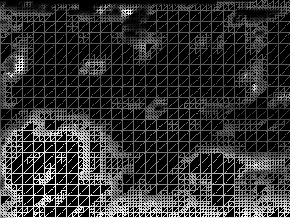
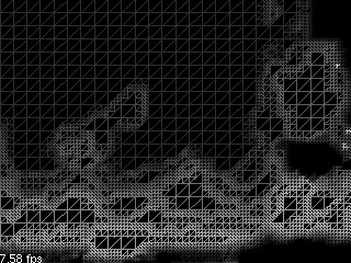
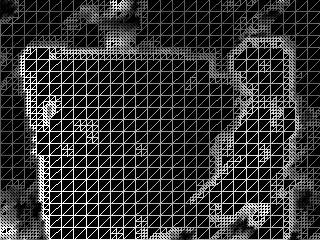
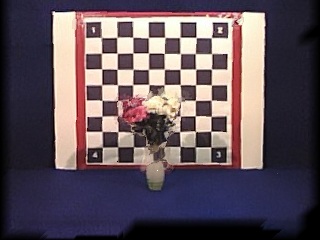
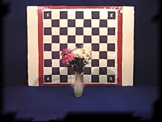
The above figures compares the rendering of a scene assuming a constant depth and our algorithm. The former algorithm was used in the MIT distributed light field camera but did not yield satisfactory results. Figure (i) is about the scene toys; Figure (ii) depicts the train scene ; Figure (iii) is what we refer to as the girl and checkerboard scene and Figure (iv) is the girl and flowers scene . Figure (a), (b) and (c) assume the depth is constant and approximately equal to the depth of the background, middle and the front objects, respectively. Due to large variation in relative scene depth, not all objects can be in focus. Figure (d) is the result of our algorithm; (e) is the multi-resolution mesh representation reconstructed on the fly (the brighter the color, the closer the scene).
The proposed algorithm handles JPEG decoding, lens distortion correction, geometry reconstruction and rendering on one of the processors of the computer. We achieve 5-10 fps for the rendering, which satisfactorily renders moderate objects traveling at a modest velocity. Some video sequences of dynamic scene rendering can be seen below. Notice that all the views in the videos are synthesized (there is no physical camera where the scene is rendered).
 The train scene (4.0 MB QuickTime MPEG-4 format).
 The Kate scene (3.1 MB QuickTime MPEG-4 format).
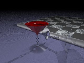
 The magic scene (12.9 MB QuickTime MPEG-4 format).
| Self-Reconfiguration of the Cameras |
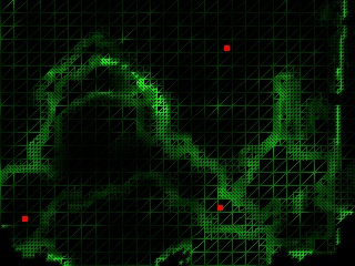
Our camera array is self-reconfigurable, which makes it possible to move the cameras in order to achieve better rendering quality. We use the inconsistency score obtained during the depth reconstruction stage to determine the new camera positions. The basic idea is to move the cameras to places where the inconsistency score is high. The following figures show the improvement of using camera rearrangement. The motion of the cameras are fully automatic based on the location of the virtual camera.
(i-a)
(ii-a)
(iii-a)
(iv-a)


(i-b)
(ii-b)
(iii-b
(iv-b)

(i-c)
(ii-c)
(iii-c)
(iv-c)
(i-d)
(ii-d)
(iii-d)
(iv-d)
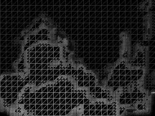
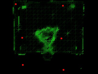
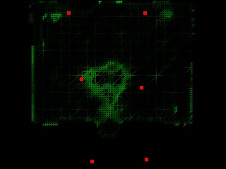
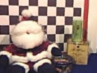
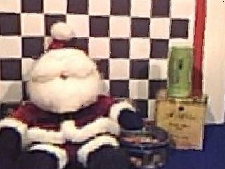
In the above figure, Figure (i) shows the scene flower, and the cameras are evenly spaced; Figure (ii) shows the same scene but the cameras are self-reconfigured; Figure (iii) shows the scene Santa, where the cameras are evenly spaced; Figure (iv) shows the result after the cameras are self-reconfigured. Figure (a) is the physical camera arrangement; Figure (b) is the reconstructed depth map, where brighter intensity means smaller depth; Figure (c) is the inconsistency score of the mesh vertices and the projection of the camera positions to the virtual imaging plane (red dots). Darker intensity means better consistency. Figure (d) is the rendered image. Notice the quality improvement from (i-d) to (ii-d) and (iii-d) to (iv-d), especially at the object boundaries.
A short video demonstrating the physical camera movement and the rendered view is listed below:
(10.6 MB QuickTime MPEG-4 format).
| Data and Code |
We provide the source code of the rendering algorithm employed in our camera array here, hoping to inspire more work along this direction. The source code package is named CAView, which stands for camera array viewer. It loads a set of images captured by an camera array and renders novel views interactively.
Download the CAView source code package
here (37 KB).
A short FAQ on CAView is available here.
The CAView program has been tested on various scenes. Some of the tested scenes are available below.
Synthetic scenes (Input images are rendered with
POV-Ray)
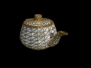
Teapot
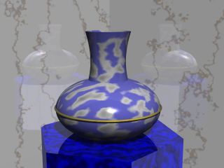
Wineglass
New skyvase
Stereo data (downloaded from the
Middlebury stereo vision
page)
Tsukuba
Cones
Teddy
Standard video sequence
Flower garden
Images captured by our camera array (most challenging
due to lens distortion, large baseline between cameras, image noise, color
variation, etc.)
Train
Toys
Kate
Show
- C. Zhang and T. Chen, "View-Dependent Non-Uniform Sampling for Image-Based Rendering", ICIP 2004.
- C. Zhang and T. Chen, "A Self-Reconfigurable Camera Array", 2004 Eurographics Symposium on Rendering 2004.
- C. Zhang and T. Chen, "A Self-Reconfigurable Camera Array", Sketch presentation in SIGGRAPH 2004.
- T. Square and T. Chen, "CMU Ultimate Eye Multi-Camera Data", MPEG April 2005
Any suggestions or comments are welcome. Please send them to Cha Zhang.